Variational Bayes Inference
Contents
3.3. Variational Bayes Inference
GTSAM is most-often used for posteriori (MAP) estimation, and with the gtsam.Marginals object we can get the Laplace approximation to the posterior density. As shown in a 2020 IJRR paper by Tim Barfoot et al, variational Bayes not only optimizes for the mean \(\mu\) but also for the covariance \(\Sigma\) of an approximation
The key is that we need to take expectations of the factor log-likelihoods with respect to \(q(x)\), and a simple way to do this is to sample from \(q\). The recipe we follow below is then:
initialize \(q(x)\) with MAP and Laplace approximation.
for a few times:
sample from q
create linearized factors using the q samples
optimize this graph
Note that we sample from \(q\), not the true posterior, which would be much harder. In the version below, which uses ancestral sampling to create the expectations, we do not need the marginals of Q explicitly, even though we do compute them in various places to draw covariance ellipses for visualization purposes.
%pip -q install gtbook # also installs latest gtsam pre-release
Note: you may need to restart the kernel to use updated packages.
import math
from math import pi, sqrt
import matplotlib.pyplot as plt
import numpy as np
from collections import defaultdict

import gtsam
import gtsam.utils.plot as gtsam_plot
from gtbook.display import show
from gtbook.display import pretty
from gtbook.gaussian import sample_bayes_net
from gtbook.driving import planar_example, marginals_figure
from gtsam import Point2, Pose2, Rot2, noiseModel
3.3.1. Sampling on the Manifold
sample_bayes_net creates samples in the tangent space, which we then need to upgrade to the non-linear manifold:
def vector_values(tangent_samples:dict, s:int):
    """Create VectorValues from sample dictionary."""
    vv = gtsam.VectorValues()
    for key in tangent_samples.keys():
        vv.insert(key, tangent_samples[key][:, s])
    return vv

def perturb(tangent_samples:dict, values:gtsam.Values, s:int, delta:None):
    """Perturb manifold values by tangent_samples[s]."""
    vv = vector_values(tangent_samples, s)
    return values.retract(vv)  if delta is None else values.retract(vv.add(delta))
3.3.2. A Simple Nonlinear Smoother Example
With the preliminaries out of the way, let us illustrate/sanity-check the GVI scheme with a simple Nonlinear smoother, having only two between constraints on Pose2 variables.
We first create the gtsam.NonlinearFactorGraph:
graph = gtsam.NonlinearFactorGraph()
x1, x2, x3 = [gtsam.symbol('x', i) for i in [1, 2, 3]]
priorMean = Pose2(0.0, 0.0, 0.0)  # prior at origin
priorNoise = noiseModel.Diagonal.Sigmas([0.1, 0.1, math.radians(1)])
graph.add(gtsam.PriorFactorPose2(x1, priorMean, priorNoise))  # add directly to graph
odometry = Pose2(2.0, 0.0, 0.0)
odometryNoise = noiseModel.Diagonal.Sigmas([0.5, 0.2, math.radians(2)])
graph.add(gtsam.BetweenFactorPose2(x1, x2, odometry, odometryNoise))
graph.add(gtsam.BetweenFactorPose2(x2, x3, odometry, odometryNoise))

# Values with ground truth
truth = gtsam.Values()
truth.insert(x1, Pose2(0, 0, 0))
truth.insert(x2, Pose2(2, 0, 0))
truth.insert(x3, Pose2(4, 0, 0))

show(graph, truth, binary_edges=True)
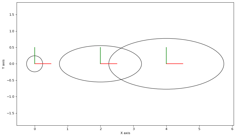
As always, we can calculate and plot covariance ellipses which show the Laplace approximation graphically.
marginals = gtsam.Marginals(graph, truth)

def make_figure():
    plt.figure(0, figsize=(12, 7), dpi=80)
    for key in [x1, x2, x3]:
        gtsam_plot.plot_pose2(0, truth.atPose2(key), 0.5,
                              marginals.marginalCovariance(key))

    plt.axis('equal')

make_figure()
We can also inspect the actual information matrix and covariance matrix, to ascertain sparsity:
def printPQ(bayes_net: gtsam.GaussianBayesNet, N:int=1):
    """Print mean, Hessian, and covariance, possibly with correction factor N"""
    R, d = bayes_net.matrix()
    Q = (R.T @ R)/N  # Hessian/Information matrix
    display(bayes_net.optimize())
    print(f"Q sparsity:\n{(Q>1e-9).astype(int)}")
    print(f"P:\n{np.round(np.linalg.inv(Q),3)}")

printPQ(graph.linearize(truth).eliminateSequential())
| Variable | value |
|---|---|
| x1 | 0 0 0 |
| x2 | 0 0 0 |
| x3 | 0 0 0 |
Q sparsity:
[[1 0 0 0 0 0 0 0 0]
 [0 1 1 0 0 0 0 0 0]
 [0 1 1 0 0 0 0 0 0]
 [0 0 0 1 0 0 0 0 0]
 [0 0 0 0 1 1 0 0 0]
 [0 0 0 0 1 1 0 0 0]
 [0 0 0 0 0 0 1 0 0]
 [0 0 0 0 0 0 0 1 0]
 [0 0 0 0 0 0 0 0 1]]
P:
[[ 0.01   0.     0.     0.01   0.     0.     0.01   0.     0.   ]
 [ 0.     0.01  -0.     0.     0.01  -0.     0.     0.01  -0.   ]
 [ 0.    -0.     0.     0.     0.001  0.     0.     0.001  0.   ]
 [ 0.01   0.     0.     0.26   0.     0.     0.26   0.     0.   ]
 [ 0.     0.01   0.001  0.     0.051  0.001  0.     0.052  0.001]
 [ 0.    -0.     0.     0.     0.001  0.002  0.     0.004  0.002]
 [ 0.01   0.     0.     0.26   0.     0.     0.51   0.     0.   ]
 [-0.     0.01   0.001 -0.     0.052  0.004 -0.     0.1    0.004]
 [ 0.    -0.     0.     0.     0.001  0.002  0.     0.004  0.003]]
3.3.3. Variational Bayes
The code below then uses this sampler to create samples on the product manifold, each sample yielding linearized factors at the sample, yielding a new Gaussian factor graph which has \(N\) times as many factors. We then optimize that graph and iterate:
N = 1000

# Start with ground truth
values = gtsam.Values(truth)

big_graph = graph.linearize(values)  # first time it's small!
bayes_net = big_graph.eliminateSequential()
delta = bayes_net.optimize()

make_figure()

for it in range(5):
    # Use the Bayes net to sample from q:
    # KEY STEP: subtract delta from Gaussian samples as we moved to new tangent space
    tangent_samples = sample_bayes_net(bayes_net, N)
    mean_correction = delta.scale(-1)
    manifold_samples = [
        perturb(tangent_samples, values, s, mean_correction) for s in range(N)]

    # Add new linearized factors for every sample:
    big_graph = gtsam.GaussianFactorGraph()
    for manifold_sample in manifold_samples:
        # KEY STEP: factors are duplicated, linearized at manifold_sample
        # TODO: *technically* these are at different tangent spaces
        sample_graph = graph.linearize(manifold_sample)
        big_graph.push_back(sample_graph)

    # Solve by calculating Bayes net and solve.
    # KEY STEP: this forms all Barfoot's expected quantities
    bayes_net = big_graph.eliminateSequential()
    delta = bayes_net.optimize()
    print(f"it {it+1}, norm of delta: {np.linalg.norm(delta.vector()):0.4f}")
    # display(delta)
    # printPQ(bayes_net)

    # update non-linear estimate
    values = values.retract(delta)
    for key in [x1, x2, x3]:
        gtsam_plot.plot_pose2(0, values.atPose2(key), 0.5)

# show new covariances
new_marginals = gtsam.Marginals(big_graph, values)
for key in [x1, x2, x3]:
    gtsam_plot.plot_pose2(0, values.atPose2(key), 0.5,
                          N*new_marginals.marginalCovariance(key))
it 1, norm of delta: 0.0401
it 2, norm of delta: 0.0401
it 3, norm of delta: 0.0015
it 4, norm of delta: 0.0013
it 5, norm of delta: 0.0017
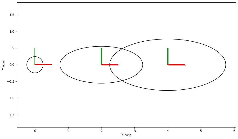
This is not converging.
3.3.4. Setting up a non-linear SLAM Example
Below we re-create a similar factor graph as in PlanarSLAMExample, but with highly nonlinear measurements on the landmarks. Take a look at the sampling example to appreciate how non-Gaussian the posteriors are in this example.
graph, truth, keys = planar_example()
x1, x2, x3, l1, l2 = keys
show(graph, truth, binary_edges=True)
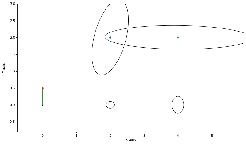
As always, we can calculate and plot covariance ellipses which show the Laplace approximation graphically.
marginals = gtsam.Marginals(graph, truth)
marginals_figure(truth, marginals, keys)
3.3.5. Variational Bayes
The code below then uses this sampler to create samples on the product manifold, each sample yielding linearized factors at the sample, yielding a new Gaussian factor graph which has \(N\) times as many factors. We then optimize that graph and iterate:
N = 1000

# Start with ground truth
values = gtsam.Values(truth)

big_graph = graph.linearize(values)  # first time it's small!
bayes_net = big_graph.eliminateSequential()
delta = bayes_net.optimize()

marginals_figure(truth, marginals, keys)
evolution = {x1: [gtsam.Point2(0, 0)], x2: [gtsam.Point2(2, 0)], x3: [
    gtsam.Point2(4, 0)], l1: [gtsam.Point2(2, 2)], l2: [gtsam.Point2(4, 2)]}

for it in range(10):
    # Use the Bayes net to sample from q:
    tangent_samples = sample_bayes_net(bayes_net, N)
    mean_correction = delta.scale(-1)
    manifold_samples = [perturb(tangent_samples, values, s, mean_correction) for s in range(N)]

    # Add new linearized factors for every sample:
    big_graph = gtsam.GaussianFactorGraph()
    for manifold_sample in manifold_samples:
        sample_graph = graph.linearize(manifold_sample)
        big_graph.push_back(sample_graph)

    # # Add Levenberg-Marquardt-style prior on delta
    if True:
        _lambda = 0.01
        for key in [x1, x2, x3]:
            big_graph.add(gtsam.JacobianFactor(key, np.eye(3), np.zeros((3,)),
                noiseModel.Isotropic.Sigma(3, _lambda)))
        for key in [l1, l2]:
            big_graph.add(gtsam.JacobianFactor(key, np.eye(2), np.zeros((2,)),
                noiseModel.Isotropic.Sigma(2, _lambda)))

    # Solve by calculating Bayes net and solving:
    bayes_net = big_graph.eliminateSequential()
    delta = bayes_net.optimize()
    print(f"it {it+1}, norm of delta: {np.linalg.norm(delta.vector()):.4f}")
    # display(delta)
    # printPQ(bayes_net)

    # update non-linear estimate
    values = values.retract(delta)

    # Record evolution
    iterate = values.retract(delta)
    for key in [x1, x2, x3]:
        evolution[key].append(iterate.atPose2(key).translation())
    for key in [l1, l2]:
        evolution[key].append(iterate.atPoint2(key))

# show evolution:
for key in [x1, x2, x3, l1, l2]:
    points = np.array(evolution[key]).T
    plt.plot(points[0], points[1])

# update non-linear estimate
final = values.retract(delta)

# show new covariances
new_marginals = gtsam.Marginals(big_graph, final)
for key in [x1, x2, x3]:
    gtsam_plot.plot_pose2(0, final.atPose2(key), 0.5,
                        N*new_marginals.marginalCovariance(key))
for key in [l1, l2]:
    gtsam_plot.plot_point2(0, final.atPoint2(key), 0.5,
                        N*new_marginals.marginalCovariance(key))

plt.show()
it 1, norm of delta: 0.1823
it 2, norm of delta: 0.1229
it 3, norm of delta: 0.0312
it 4, norm of delta: 0.0182
it 5, norm of delta: 0.0126
it 6, norm of delta: 0.0088
it 7, norm of delta: 0.0062
it 8, norm of delta: 0.0044
it 9, norm of delta: 0.0031
it 10, norm of delta: 0.0023
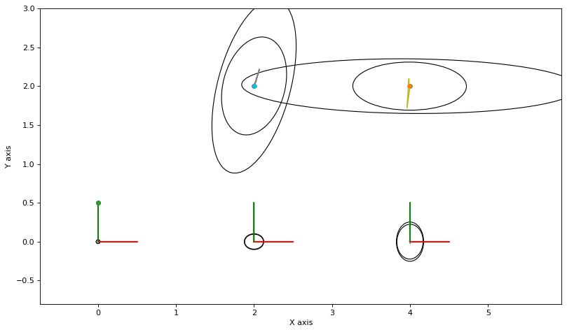
3.3.6. Compared with MCMC
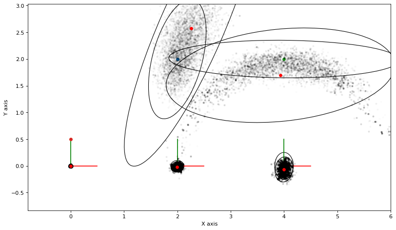
The above converges but is very conservative. The culprit seems to be either (a) a bug in the implementation above, or (b) more likely, that the Kullback-Leibler divergence \(D_\text{KL}(q\|p)\) is a poor approximation scheme in this case.
If we use MCMC sampling instead, and fit Gaussian densities to the samples, we get a very different answer:
markov_blankets = defaultdict(gtsam.NonlinearFactorGraph)
for i in range(graph.size()):
    factor = graph.at(i)
    for j in factor.keys():
        markov_blankets[j].add(factor)

def accept(log_a):
    """calculate acceptance, with some care to avoid overflow."""
    if log_a >= 0:
        return True
    if log_a < -10:
        return False
    return np.random.uniform() < math.exp(log_a)

def plot_sample(manifold_sample, alpha=0.1):
    points = np.empty((2, 5))
    for i in [1, 2, 3]:
        points[:,i-1] = manifold_sample.atPose2(gtsam.symbol('x', i)).translation()
    for j in [1, 2]:
        points[:,j+2] = manifold_sample.atPoint2(gtsam.symbol('l', j))
    plt.plot(points[0], points[1], 'k.', markersize=5, alpha=alpha)
    return points

marginals_figure(truth, marginals, keys)
N = 50000
stats = []
nr_accepted = 0
gbn = graph.linearize(truth).eliminateSequential()
tangent_proposals = sample_bayes_net(gbn, N)

# Start with an initial estimate x
x = gtsam.Values(truth)
for s in range(N):
    # choose a variable to perturb
    j = keys[np.random.choice(5)]
    vvj = gtsam.VectorValues()
    vvj.insert(j, tangent_proposals[j][:, s])
    p = x.retract(vvj)
    # calculate local acceptance ratio
    log_a = markov_blankets[j].error(x) - markov_blankets[j].error(p)
    if accept(log_a):
        nr_accepted += 1
        x = p
        stats.append(plot_sample(x, alpha=0.01))

print(f"{nr_accepted=}")

# estimate Gaussian params
stats_tensor = np.array(stats)
mean = stats_tensor.mean(axis=0)
for j in range(5):
    centered = stats_tensor[:,:,j] - mean[:,j]
    P = (centered.T @ centered)/(nr_accepted-1)
    gtsam_plot.plot_point2(0, mean[:,j], 'r', P)

plt.show()
nr_accepted=15123
