Loopy Belief Propagation
Contents
1.4. Loopy Belief Propagation
We start from the same “image MRF, with unary and pairwise Gaussian factors. We then implement loopy belief propagation.
%pip -q install gtbook # also installs latest gtsam pre-release
Note: you may need to restart the kernel to use updated packages.
import math
import numpy as np
from collections import defaultdict
import plotly.express as px
from plotly.subplots import make_subplots
import plotly.graph_objects as go

try:
    import google.colab
except:
    import plotly.io as pio
    pio.renderers.default = "png"

import gtsam
from gtbook.display import show
from gtsam import noiseModel

def square(vv):
    result = gtsam.VectorValues()
    for k in key_list:
        result.insert(k, vv.at(k)**2)
    return result
1.4.1. A Small “Image” MRF
All the code to create the small image “MRF” in one cell:
M, N = 3, 4  # try playing with this
row_symbols = [chr(ord('a')+row) for row in range(M)]
keys = {(row, col): gtsam.symbol(row_symbols[row], col+1)
       for row in range(M) for col in range(N)}

sigma = 0.5
rng = np.random.default_rng(42)
data = rng.normal(loc=0, scale=sigma, size=(M, N, 1))
data_model = noiseModel.Isotropic.Sigmas([sigma])

smoothness_sigma = 0.5
smoothness_model = noiseModel.Isotropic.Sigmas([smoothness_sigma])

I = np.eye(1, 1, dtype=float)
zero = np.zeros((1,1))
graph = gtsam.GaussianFactorGraph()
for row in range(M):
    for col in range(N):
        # add data terms:
        j = keys[(row,col)]
        graph.add(j, I, np.array(data[row,col]), data_model)
        # add smoothness terms:
        if col>0:
            j1 = keys[(row,col-1)]
            graph.add(j, I, j1, -I, zero, smoothness_model)
        if row>0:
            j2 = keys[(row-1,col)]
            graph.add(j, I, j2, -I, zero, smoothness_model)

position_hints = {c:float(1-i) for i,c in enumerate(row_symbols)}
show(graph, binary_edges=True, hints=position_hints)
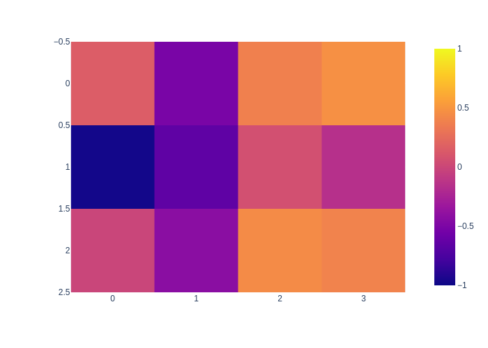
And the data image is shown here:
px.imshow(data[:,:,0], zmin=-1, zmax=1)

1.4.2. Loopy Belief Propagation
We initialize a set of individual Gaussian factors \(q(x_j)\) or beliefs, one for each variable. LBP is a fixed point algorithm to minimize the KL \(D_\text{KL}(p||q)\) divergence between the true posterior \(p(X|Z)\) and the variational approximation
We repeatedly:
pick a variable \(x_j\) at random;
consider the Markov blanket of \(x_j\), the factor graph fragment \(\phi(x_j, X_j)\) where \(X_j\) is the separator;
augment the factor graph fragment with (downdated) beliefs on all \(x_k\in X_j\), except \(q(x_j)\);
eliminate the separator \(X_j\) by factorizing this graph as \(p(X_j|x_j)q'(x_j)\);
assign \(q(x_j) \leftarrow q'(x_j)\) to be the new belief on \(x_j\).
We first cache all Markov blankets:
local_factor_indices =  defaultdict(list)
markov_blankets = defaultdict(gtsam.GaussianFactorGraph)
for i in range(graph.size()):
    factor = graph.at(i)
    for j in factor.keys():
        local_factor_indices[j].append(i)
        markov_blankets[j].add(factor)
Here are the Markov blanket for \(x_{a1}\) and \(x_{b2}\):
show(markov_blankets[keys[0,0]], binary_edges=True, hints=position_hints)
show(markov_blankets[keys[0,1]], binary_edges=True, hints=position_hints)
We store the belief \(q(x)\) as gtsam.GaussianDensity instances. The entire LPB code is then:
def lbp(x0: gtsam.VectorValues, hook=None, max_iterations=100, seed=42, initial_sigma=5.0):
    """Perform loopy belief propagation with initial estimate x."""
    key_list = list(keys.values())

    # Initialize belief
    q = {j: gtsam.GaussianDensity.FromMeanAndStddev(
        j, x0.at(j), initial_sigma) for j in key_list}

    # Initialize messages from factor i to variable j
    z = np.zeros((1, 1), float)
    messages = {i: {j: gtsam.HessianFactor(j, z, z, 0)
                    for j in key_list} for i in range(graph.size())}

    def get_message(i: int, j: int):
        """Get message from factor to j"""
        factor = graph.at(i)
        if factor.size() == 1: return factor
        factor_graph, ordering = gtsam.GaussianFactorGraph(), gtsam.Ordering()
        factor_graph.push_back(factor)
        for k in [l for l in factor.keys() if l != j]:
            ordering.push_back(k)
            factor_graph.add(q[k])
            factor_graph.add(messages[i][k].negate())  # downdates!
        _, remaining = factor_graph.eliminatePartialSequential(ordering)
        return remaining.at(0)

    def update(j: int):
        """Augment Markov blanket and eliminate to x_j"""
        # Calculate "messages" from all factors in Markov blanket:
        augmented_graph = gtsam.GaussianFactorGraph()
        for i in local_factor_indices[j]:
            messages[i][j] = get_message(i, j)
            augmented_graph.push_back(messages[i][j])

        # Eliminate with x_j eliminated last:
        ordering = gtsam.Ordering.ColamdConstrainedLastGaussianFactorGraph(
            augmented_graph, [j])
        gbn = augmented_graph.eliminateSequential(ordering)
        q[j] = gbn.back()  # new belief!

    hook(0, None, q)
    rng = np.random.default_rng(seed)
    for it in range(1, max_iterations+1):
        # choose a variable whose belief to update
        j = key_list[rng.choice(M*N)]
        update(j)
        hook(it, j, q)
    return q
We initialize to the data:
rng = np.random.default_rng(42)
initial = gtsam.VectorValues()
for row in range(M):
    for col in range(N):
        j = keys[(row,col)]
        initial.insert(j, data[row,col])
def calculate_mean(q):
    """Calculate mean of each q[j]"""
    mean = gtsam.VectorValues()
    for j, qj in q.items():
        mean.insert(j, q[j].solve(mean).at(j))
    return mean

def print_hook(it, j, q):
    error = graph.error(calculate_mean(q))
    if it % 10 == 0:
        if it==0:
            print(f"{it=}, initial error is {error}")
        else:
            print(f"{it=}, updated {gtsam.DefaultKeyFormatter(j)}, error now {error}")

q = lbp(initial, print_hook, max_iterations=150)
it=0, initial error is 12.126645986142575
it=10, updated a2, error now 9.113900486816643
it=20, updated b2, error now 8.524714446372975
it=30, updated b2, error now 4.881997061292955
it=40, updated b4, error now 3.3732148265768735
it=50, updated c2, error now 3.191536790242739
it=60, updated c1, error now 3.147855313649847
it=70, updated b2, error now 3.1464772839425956
it=80, updated c1, error now 3.1456805402875254
it=90, updated c2, error now 3.14452888223852
it=100, updated a2, error now 3.1442569269735574
it=110, updated c1, error now 3.1441842205421846
it=120, updated a2, error now 3.144144868279104
it=130, updated b4, error now 3.1441466837532785
it=140, updated b2, error now 3.1441423296105064
it=150, updated a1, error now 3.144001745678235
We compare the mean with the exact mean and see that LBP converges to the correct mean value:
x = calculate_mean(q)
stddev = np.empty((M*N,))
for i, (j,qj) in enumerate(q.items()):
    information = qj.information().item()
    stddev[i] = 1.0/math.sqrt(information)
    print(f"{gtsam.DefaultKeyFormatter(j)} {x.at(j).item():.2f} +/- {stddev[i]:.2f}")
a1 -0.16 +/- 0.32
a2 -0.22 +/- 0.28
a3 0.09 +/- 0.28
a4 0.21 +/- 0.32
b1 -0.41 +/- 0.29
b2 -0.30 +/- 0.25
b3 0.00 +/- 0.25
b4 0.06 +/- 0.29
c1 -0.21 +/- 0.32
c2 -0.21 +/- 0.28
c3 0.11 +/- 0.28
c4 0.18 +/- 0.32
The exact mean is calculated below, as well as the exact standard deviations.
key_list = list(keys.values())
bayes_tree = graph.eliminateMultifrontal()
exact_mean = bayes_tree.optimize()
exact_stddev = np.empty((M*N,))
for i, j in enumerate(key_list):
    variance = bayes_tree.marginalCovariance(j)
    exact_stddev[i] = math.sqrt(variance)
    print(f"{gtsam.DefaultKeyFormatter(j)} {exact_mean.at(j).item():.2f} +/- {exact_stddev[i]:.2f}")
print(f"direct solver error: {graph.error(exact_mean)}")
a1 -0.16 +/- 0.33
a2 -0.22 +/- 0.29
a3 0.09 +/- 0.29
a4 0.21 +/- 0.33
b1 -0.41 +/- 0.29
b2 -0.30 +/- 0.26
b3 0.00 +/- 0.26
b4 0.06 +/- 0.29
c1 -0.21 +/- 0.33
c2 -0.21 +/- 0.29
c3 0.11 +/- 0.29
c4 0.18 +/- 0.33
direct solver error: 3.1439968801524447
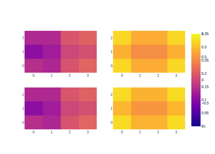
As you can see, the LBP approximation is a bit over-confident. This is a well known property of LBP. we show the effect side by side again below, with LBP \(\mu/\sigma\) in the top row, and exact \(\mu/\sigma\) in the bottom row.
fig = make_subplots(rows=2, cols=2)
fig.add_trace(go.Heatmap(z=x.vector().reshape((M, N)), zmin=-1, zmax=1), row=1, col=1)
fig.add_trace(go.Heatmap(z=exact_mean.vector().reshape((M, N)), zmin=-1, zmax=1), row=2, col=1)
fig.add_trace(go.Heatmap(z=stddev.reshape((M, N)), zmin=0, zmax=0.35), row=1, col=2)
fig.add_trace(go.Heatmap(z=exact_stddev.reshape((M, N)), zmin=0, zmax=0.35), row=2, col=2)
fig.show()

1.4.3. Gibbs Sampling
Gibbs sampling is a variant of Markov Chain Monte Carlo sampling that always accepts any proposal.
We repeatedly:
pick a variable \(x_j\) at random;
consider the Markov blanket of \(x_j\), the factor graph fragment \(\phi(x_j, X_j)\) where \(X_j\) is the separator;
eliminate the variable \(x_j\) by factorizing \(\phi(x_j, X_j) = p(x_j|X_j)\phi(X_j)\);
sample \(x_j\) \(\phi(x_j, X_j)\).
We first compute all conditionals \(p(x_j|X_j)\), which we can do in advance, as well as the inverse square root covariances \(R_j^{-1}\), which we need for sampling. An advantage of working in square-root information form (like the entirety of GTSAM) is that less computation is needed and it is numerically more stable:
conditionals = {}
invR = {}
for j in key_list:
    local_graph = markov_blankets[j]
    # Eliminate just x_j:
    ordering = gtsam.Ordering()
    ordering.push_back(j)
    gbn, _ = local_graph.eliminatePartialSequential(ordering)
    conditionals[j] = gbn.at(0)
    invR[j] = np.linalg.inv(conditionals[j].R())
The conditional is parameterized by \(R\), \(S\) and \(d\) as follows:
A Gibbs proposal for variable \(j\) then just assembles the separator \(X_j\) and samples from the conditional like so:
where \(\mu(X_j) = R_j^{-1} [d - S X_j]\) is the conditional mean and \(u\) is drawn from a standard zero-mean Gaussian with identity covariance.
rng = np.random.default_rng(42)

def proposal(x, j):
    """Propose via Gibbs sampling"""
    # Get Conditional for x_j, computed above
    conditional = conditionals[j]
    # sample x_j and propose a new sample
    rhs = conditional.d().reshape(1, 1)
    key, *parents = conditional.keys()
    rhs = rhs - conditional.S() @ np.vstack([x.at(p) for p in parents])
    # sample from conditional Gaussian
    sample = gtsam.VectorValues()
    sample.insert(j, invR[j] @ (rhs + rng.normal()))
    new_x = gtsam.VectorValues(x)
    new_x.update(sample)
    return new_x
We also create a hook to keep sufficient statistics:
global count, sum, sum_squares
count = 0
sum = gtsam.VectorValues.Zero(initial)
sum_squares = gtsam.VectorValues.Zero(initial)

def save_stats(it, y):
    global count, sum, sum_squares
    count += 1
    sum = sum.add(y)
    sum_squares = sum_squares.add(square(y))
The Gibbs sampler is then exceedingly simple:
# run Gibbs sampler
nr_iterations = M*N*5000
y = gtsam.VectorValues(initial)
for it in range(nr_iterations):
    j = key_list[rng.choice(M*N)] # choose a variable to perturb
    y = proposal(y, j)
    if it >= nr_iterations//2: save_stats(it, y)
Because we kept the sufficient statistics count, sum, and sum_squares we can compute the marginals:
gibbs_mean = sum.scale(1.0/count)
avg_deviation = sum_squares.scale(1.0/count)
variance = avg_deviation.subtract(square(gibbs_mean))

print(f"Marginals computed from {count} correlated samples:")
gibbs_stddev = np.empty((M*N,))
for i, j in enumerate(key_list):
    gibbs_stddev[i] = math.sqrt(variance.at(j))
    print(f"{gtsam.DefaultKeyFormatter(j)} {gibbs_mean.at(j).item():.2f} +/- {gibbs_stddev[i]:.2f}")
print(f"The error at the mean is {graph.error(gibbs_mean)}.")
Marginals computed from 30000 correlated samples:
a1 -0.14 +/- 0.33
a2 -0.21 +/- 0.29
a3 0.11 +/- 0.29
a4 0.20 +/- 0.33
b1 -0.40 +/- 0.30
b2 -0.29 +/- 0.25
b3 0.02 +/- 0.26
b4 0.05 +/- 0.30
c1 -0.22 +/- 0.33
c2 -0.20 +/- 0.30
c3 0.11 +/- 0.29
c4 0.17 +/- 0.34
The error at the mean is 3.150451230285521.
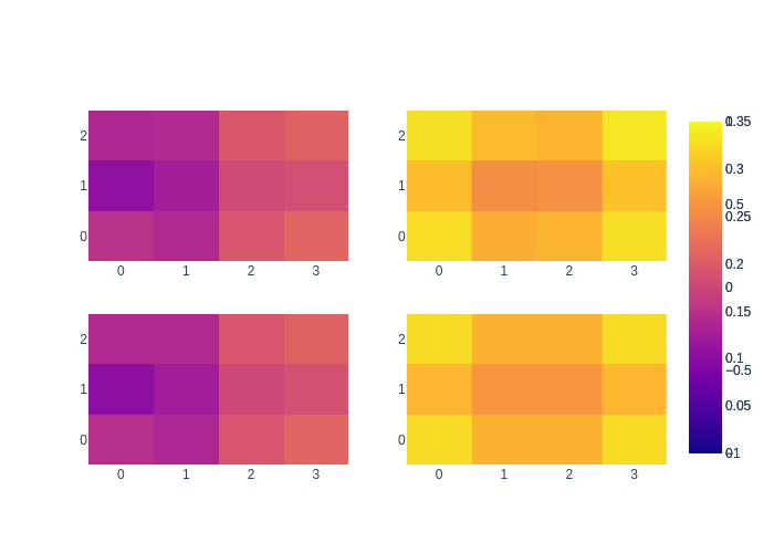
Comparing these with the direct solver solution above you can see that the mean converges, as well as the standard deviations. We also show this graphically below:
fig = make_subplots(rows=2, cols=2)
fig.add_trace(go.Heatmap(z=gibbs_mean.vector().reshape((M, N)), zmin=-1, zmax=1), row=1, col=1)
fig.add_trace(go.Heatmap(z=exact_mean.vector().reshape((M, N)), zmin=-1, zmax=1), row=2, col=1)
fig.add_trace(go.Heatmap(z=gibbs_stddev.reshape((M, N)), zmin=0, zmax=0.35), row=1, col=2)
fig.add_trace(go.Heatmap(z=exact_stddev.reshape((M, N)), zmin=0, zmax=0.35), row=2, col=2)
fig.show()

1.4.4. Elimination vs. Message Passing
Above we implemented LBP with elimination, where the root of the eliminated graph becomes the new belief \(q_j(x_j)\). The duality with Gibbs sampling is clear, and it is very natural if you are familiar with the elimination on factor graphs.
However, LBP is traditionally explained/implemented with a more complex “message passing” algorithm, with two different types of messages (variable to factor, and factor to variable). Are they in fact the same? Using the small example for the top-left pixel below we will show that they are indeed.
Below we show the Markov blanket for \(a1\), which has three factors. Let us name the unary factor \(f_{a1}\), and the binary factors \(f_{a2}\) and \(f_{b1}\):
show(markov_blankets[keys[0,0]], binary_edges=True, hints=position_hints)
On this very cool tutorial from Imperial college the more traditional view is explained beautifully. Three messages would be sent to \(a1\) from the three factors:
which are then combined in the belief update
The variable to factor messages \(m_{x\rightarrow f} (x)\) are calculated as the beliefs, down-dated by the last message \(m_{f\rightarrow x} (x)\) from \(f\) to \(x\):
This is slightly different from the traditional exposition, but equivalent. Hence the final belief update is
LBP implemented by elimination yields obtains a new belief for \(a1\) by factorizing the Markov blanket, augmented with downdated beliefs \(\frac{q(a2)}{m_{f_{a2}\rightarrow a2} (a2)}\) and \(\frac{q(b1)}{m_{f_{b1}\rightarrow b1} (b1)}\):
where \(q(a1)\) is obtained by marginalizing out \(a2\) and \(b1\):
This is exactly the same.
