1.1. Kalman Smoother¶

GTSAM is based on sparse factorization, which it implements by elimination of a Gaussian factor graph. A Kalman smoother is a simple linear Markov chain, with Gaussian measurements and Gaussian Motion models, and as a result GTSAM simply eats through it, like a knife through butter.

%pip -q install gtbook # also installs latest gtsam pre-release

Note: you may need to restart the kernel to use updated packages.

import math
import matplotlib.pyplot as plt
import numpy as np

import gtsam
import gtsam.utils.plot as gtsam_plot
from gtbook.display import show
from gtbook.gaussian import sample_bayes_net
from gtsam import Point2, noiseModel

# Some keys we use below:
x1, x2, x3 = [gtsam.symbol('x', i) for i in [1, 2, 3]]

1.1.1. A Simple Kalman Smoother Example¶

We illustrate this with a simple 3-state Kalman smoother. It also shows how the solution the Kalman smoother is a Bayes net, which exactly captures the Gaussian posterior.

We first set up a small GaussianFactorGraph. I like specifying factors in this case with a gtsam.JacobianFactor:

gfg = gtsam.GaussianFactorGraph()

# add "measurements" |x1|^2, |x2-(2,0)|^2, |x3-(4,0)|^2
model2 = noiseModel.Isotropic.Sigma(2, 0.5)
I2 = np.eye(2, dtype=float)
for i, key in enumerate([x1, x2, x3]):
    gfg.add(gtsam.JacobianFactor(i1=key, A1=I2,
            b=gtsam.Point2(i*2, 0), model=model2))  # prior

# add "motion models" |x2 - x1 - (2,0)|^2, |x3 - x2 - (2,0)|^2
motion_model = noiseModel.Diagonal.Sigmas([0.1,0.3])
for i1, i2 in [(x1, x2), (x2, x3)]:
    gfg.add(gtsam.JacobianFactor(i1=i1, A1=-I2, i2=i2, A2=I2,
            b=gtsam.Point2(2, 0), model=motion_model))  # between x1 and x2

show(gfg)

Solving this with GTSAM is trivial, and because in this case the measurements and motion models agree perfectly, the solution has zero error:

smoother_solution = gfg.optimize()
print(f"solution = {smoother_solution} with error {gfg.error(smoother_solution):.2f}")

solution = VectorValues: 3 elements
  x1: 2.43861e-15           0
  x2: 2 0
  x3: 4 0
 with error 0.00

1.1.2. The Posterior as a Bayes Net¶

The way GTSAM solves this is by eliminating \(x_1\), then \(x_2\), and then \(x_3\), yielding a Bayes net made up of Gaussian Conditionals. We can call eliminateSequential to obtain the Bayes net to visualize it:

gbn = gfg.eliminateSequential()
show(gbn)

The Bayes net is equivalent to an upper triangular matrix \(R\), which we can explicitly produce. This produces a dense matrix, but that’s OK in this small example:

R, d = gbn.matrix()
print(np.round(R,2))

[[10.2   0.   -9.81  0.    0.    0.  ]
 [ 0.    3.89  0.   -2.86  0.    0.  ]
 [ 0.    0.   10.38  0.   -9.63  0.  ]
 [ 0.    0.    0.    4.25  0.   -2.62]
 [ 0.    0.    0.    0.    3.36  0.  ]
 [ 0.    0.    0.    0.    0.    2.88]]

The \(d\) above is the “square root information vector”, as the Bayes net defines the following quadratic, and corresponding Gaussian density, in this case in \(\mathbb{R}^6\):

\[ E_{gbn}(x; R, d) \doteq \frac{1}{2} \|Rx - d\|^2 \]

\[ \mathcal{N}_{gbn}(x; R, d) \sim k \exp \{- \frac{1}{2} \|Rx - d\|^2\} \]

1.1.3. Marginals, the Hard Way¶

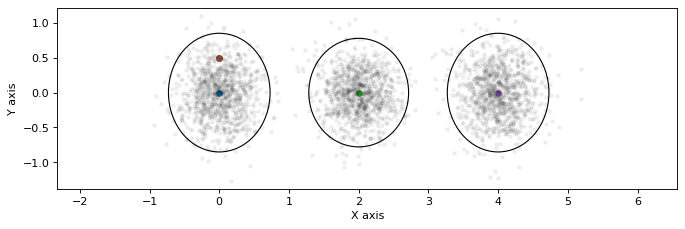
The mean of this Gaussian is \(\mu=R^{-1}d\) and its covariance \(P=(R^TR)^{-1}\). The latter allows us to obtain and plot the marginals:

P = np.linalg.inv(R.T @ R) # full 6*6 covariance matrix

def gaussian_figure():
    plt.figure(0, figsize=(10, 3), dpi=80)
    for i, key in enumerate([x1, x2, x3]):
        gtsam_plot.plot_point2(0, smoother_solution.at(key), 0.5, P[i*2:(i+1)*2,i*2:(i+1)*2])

    plt.axis('equal')

gaussian_figure()

1.1.4. Efficient Marginals using the Bayes Tree¶

The above approach to obtain the covariance \(P\) is very expensive if \(x\) is high dimensional. Note that there are better ways to obtain the marginals, and this is implemented by the Bayes tree, which we can obtain by multi-frontal elimination instead:

bayes_tree = gfg.eliminateMultifrontal()
show(bayes_tree)

The above shows the Bayes tree, which is a directed tree of cliques. The undirected version of this is known as the clique tree or junction tree. One of the “hidden secrets” of GTSAM is that it has a very efficient way of calculating the marginals in a Bayes tree:

for key in [x1,x2,x3]:
    print(f"{gtsam.DefaultKeyFormatter(key)}:\n{bayes_tree.marginalCovariance(key)}\n")

x1:
[[0.08868927 0.        ]
 [0.         0.12088585]]

x2:
[[0.08552632 0.        ]
 [0.         0.10119048]]

x3:
[[0.08868927 0.        ]
 [0.         0.12088585]]

It can even compute arbitrary joint marginals for any two variables:

Q, _ = bayes_tree.joint(x1,x3).hessian()
print(np.linalg.inv(Q))

[[0.08868927 0.         0.07907389 0.        ]
 [0.         0.12088585 0.         0.05470938]
 [0.07907389 0.         0.08868927 0.        ]
 [0.         0.05470938 0.         0.12088585]]

1.1.5. Sampling¶

Bayes nets support efficient ancestral sampling, which produces samples from the joint as a dictionary:

for key, sample in sample_bayes_net(gbn, 5).items():
    print(f"{gtsam.DefaultKeyFormatter(key)}:\n{sample}")

x3:
[[ 4.10309098  4.02855232  4.55185471  4.42654043  3.59527439]
 [-0.22051105 -0.00774796 -0.43506119  0.32430253  0.27281872]]
x2:
[[ 2.18632111  2.07574816  2.53918228  2.47804704  1.68996933]
 [-0.31487864 -0.12062116 -0.56571078 -0.34220257  0.17401268]]
x1:
[[ 0.17095927  0.06197369  0.60020091  0.3963372  -0.29111854]
 [ 0.01430849 -0.09455421 -0.1405038  -0.37668028  0.2126222 ]]

It is fast, as sampling is done batch-wise, e.g., for batch-size \(N=1000\):

%%timeit
samples = sample_bayes_net(gbn, 1000)

303 µs ± 5.69 µs per loop (mean ± std. dev. of 7 runs, 1,000 loops each)

gaussian_figure()
for key, points in sample_bayes_net(gbn, 1000).items():
    plt.plot(points[0], points[1], 'k.', alpha=0.05)

1.1.6. Conclusion¶

Kalman smoothers are easy. Kalman filters are actually harder to implement, but we also did that for you, in gtsam.KalmanFilter and gtsam.ExtendedKalmanFilter.

GTSAM by Example

Kalman Smoother

Contents